Note
This tutorial was generated from a Jupyter notebook that can be downloaded here.
PTA Demo 1: Analyze reference metronome data files
The folowing demonstration notebook goes through the various commands
needed to get profiles from single metronome observations and then to
analyze the signal from double metronomes to get the correlations that
reveal the motion of the recording microphone. All of the functionality
is available in a GUI format by calling the commands
PTAdemo_single_metronome and PTAdemo_double_metronome.
Record single metronome pulses
# filenames and beats per minute
path = tpta.__path__ + '/demo_data/'
metfile1 = path + 'm208a'
metfile2 = path + 'm184b'
metfiles = path + 'm208a184b'
bpm1 = 208
bpm2 = 184
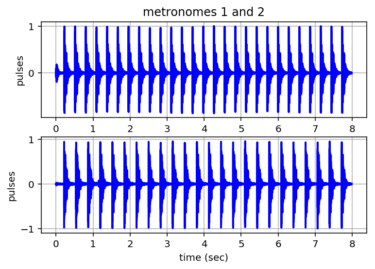
Play recorded pulses
# sample rate
Fs = 44100

# play recorded sound
ts1 = tpta.playpulses(metfile1 + ".txt")

# plot time series
plt.figure()
plt.subplot(2,1,1)
plt.plot(ts1[:,0], ts1[:,1], lw=2, color='b')
plt.ylabel('pulses')
plt.title('metronomes 1 and 2')
plt.grid('on')

# play recorded sound
ts2 = tpta.playpulses(metfile2 + ".txt")

# plot time series
plt.subplot(2,1,2)
plt.plot(ts2[:,0], ts2[:,1], lw=2, color='b')
plt.xlabel('time (sec)')
plt.ylabel('pulses')
plt.grid('on')
plt.draw()

# print to file
plt.savefig(metfiles + "_pulses.pdf", bbox_inches='tight')
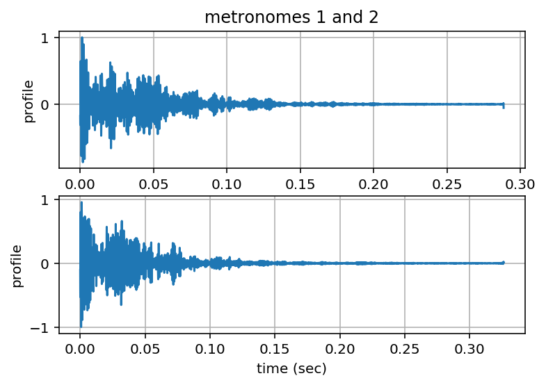
Calculate and Plot Pulse Profiles
# metronome 1
print('calculating pulse period and profile of metronome 1...')
[profile1, T1] = tpta.calpulseprofile(ts1, bpm1)
print('T1 = ', T1, 'sec')

# plot pulse profile
plt.figure()
plt.subplot(2,1,1)
plt.plot(profile1[:,0], profile1[:,1])
plt.ylabel('profile')
plt.title('metronomes 1 and 2')
plt.grid('on')

# write pulse profile to file
outfile1 = metfile1 + "_profile_nb.txt"
np.savetxt(outfile1, profile1)

# metronome 2
print('calculating pulse period and profile of metronome 2...')
[profile2, T2] = tpta.calpulseprofile(ts2, bpm2)
print('T2 = ', T2, 'sec')

# plot pulse profile
plt.subplot(2,1,2)
plt.plot(profile2[:,0], profile2[:,1])
plt.xlabel('time (sec)')
plt.ylabel('profile')
plt.grid('on')
plt.draw()

# write pulse profile to file
outfile2 = metfile2 + "_profile_nb.txt"
np.savetxt(outfile2, profile2)

# print to file
plt.savefig(metfiles + "_profilesb_n.pdf", bbox_inches='tight')
calculating pulse period and profile of metronome 1...
T1 =  0.288561538462 sec
calculating pulse period and profile of metronome 2...
T2 =  0.326096956522 sec
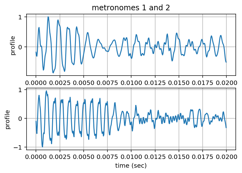
Zoom-in on Profiles
Nzoom = np.int(np.round(0.01*Fs))

plt.figure()
plt.subplot(2,1,1)
plt.plot(profile1[:Nzoom,0], profile1[:Nzoom,1])
plt.ylabel('profile')
plt.title('metronomes 1 and 2')
plt.grid('on')

plt.subplot(2,1,2)
plt.plot(profile2[:Nzoom,0], profile2[:Nzoom,1])
plt.xlabel('time (sec)')
plt.ylabel('profile')
plt.grid('on')
plt.draw()

# print to file
plt.savefig(metfiles + "_profiles_zoom.pdf", bbox_inches='tight')
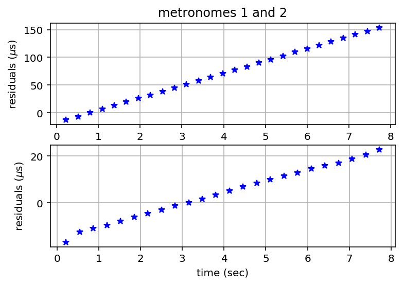
Calculate Residuals
# calculate residuals for metronome 1
template1 = tpta.caltemplate(profile1, ts1)
[measuredTOAs1, uncertainties1, n01] = tpta.calmeasuredTOAs(ts1, template1, T1)
Np1 = len(measuredTOAs1)
expectedTOAs1 = tpta.calexpectedTOAs(measuredTOAs1[n01-1], n01, Np1, T1)
[residuals1, errorbars1] = tpta.calresiduals(measuredTOAs1, expectedTOAs1, uncertainties1)

# calculate residuals for metronome 2
template2 = tpta.caltemplate(profile2, ts2)
[measuredTOAs2, uncertainties2, n02] = tpta.calmeasuredTOAs(ts2, template2, T2)
Np2 = len(measuredTOAs2)
expectedTOAs2 = tpta.calexpectedTOAs(measuredTOAs2[n02-1], n02, Np2, T2)
[residuals2, errorbars2] = tpta.calresiduals(measuredTOAs2, expectedTOAs2, uncertainties2)
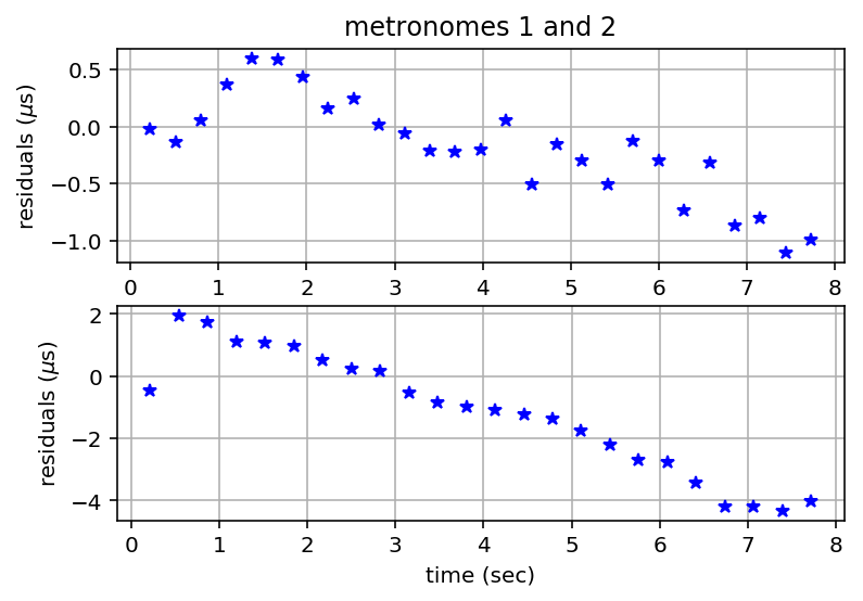
Plot Residuals
plt.figure()
plt.subplot(2,1,1)
plt.plot(residuals1[:,0], 1.e6*residuals1[:,1], 'b*');
plt.ylabel('residuals ($\mu$s)')
plt.title('metronomes 1 and 2')
plt.grid('on')

plt.subplot(2,1,2)
plt.plot(residuals2[:,0], 1.e6*residuals2[:,1], 'b*');
plt.xlabel('time (sec)')
plt.ylabel('residuals ($\mu$s)')
plt.grid('on')
plt.draw()

# print to file
plt.savefig(metfiles + "_residuals.pdf", bbox_inches='tight')
Calculate and Plot Detrended Residuals
[dtresiduals1, b, m] = tpta.detrend(residuals1, errorbars1);
N1 = len(residuals1[:,0])
T1new = T1 + m*(residuals1[-1,0]-residuals1[0,0])/(N1-1)
print("improved pulse period estimate of metronome 1 =", T1new, "sec")

[dtresiduals2, b, m] = tpta.detrend(residuals2, errorbars2);
N2 = len(residuals2[:,0])
T2new = T2 + m*(residuals2[-1,0]-residuals2[0,0])/(N2-1)
print("improved pulse period estimate of metronome 2 =", T2new, "sec")

# plot residuals
plt.figure()
plt.subplot(2,1,1)
plt.plot(dtresiduals1[:,0], 1.e6*dtresiduals1[:,1], 'b*');
plt.ylabel('residuals ($\mu$s)')
plt.title('metronomes 1 and 2')
plt.grid('on')

plt.subplot(2,1,2)
plt.plot(dtresiduals2[:,0], 1.e6*dtresiduals2[:,1], 'b*');
plt.xlabel('time (sec)')
plt.ylabel('residuals ($\mu$s)')
plt.grid('on')
plt.draw()

# print to file
plt.savefig(metfiles + "detrended_residuals.pdf", bbox_inches='tight')
improved pulse period estimate of metronome 1 = 0.288567978601 sec
improved pulse period estimate of metronome 2 = 0.32609882891 sec
PTA Demo 2 - Double-Metronome Correlations
Record Double-Metronome Data
# filenames (time-series and pulse profiles)
tsfile = 'm208a184b135'
profilefile1 = 'm208a_profile'
profilefile2 = 'm184b_profile'
T1 = T1new
T2 = T2new
#brecord pulses from both metronomes
tpta.recordpulses(tsfile + ".txt")
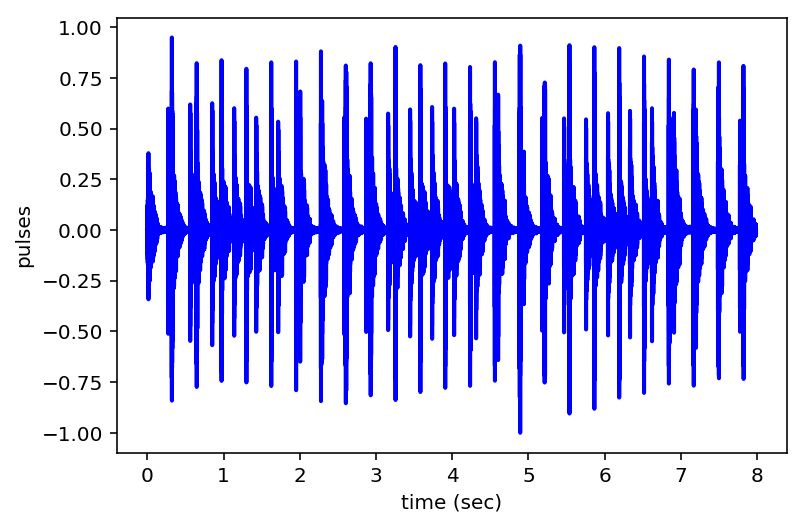
Play Recorded Pulses
# play recorded sound

ts = tpta.playpulses(path + tsfile + ".txt")

# plot time series
plt.figure()
plt.plot(ts[:,0], ts[:,1], lw=2, color='b')
plt.xlabel('time (sec)');
plt.ylabel('pulses');
plt.grid
plt.draw()

# print to file
plt.savefig(tsfile + "_pulses.pdf", bbox_inches='tight')
Calculate Residuals
# load pulse profiles
profile1 = np.loadtxt(profilefile1 + ".txt")
profile2 = np.loadtxt(profilefile2 + ".txt")

# calculate residuals for metronome 1
template1 = tpta.caltemplate(profile1, ts)
[measuredTOAs1, uncertainties1, n01] = tpta.calmeasuredTOAs(ts, template1, T1)
Np1 = len(measuredTOAs1)
expectedTOAs1 = tpta.calexpectedTOAs(measuredTOAs1[n01-1], n01, Np1, T1)
[residuals1, errorbars1] = tpta.calresiduals(measuredTOAs1, expectedTOAs1, uncertainties1)

# calculate residuals for metronome 2
template2 = tpta.caltemplate(profile2, ts)
[measuredTOAs2, uncertainties2, n02] = tpta.calmeasuredTOAs(ts, template2, T2)
Np2 = len(measuredTOAs2)
expectedTOAs2 = tpta.calexpectedTOAs(measuredTOAs2[n02-1], n02, Np2, T2)
[residuals2, errorbars2] = tpta.calresiduals(measuredTOAs2, expectedTOAs2, uncertainties2)
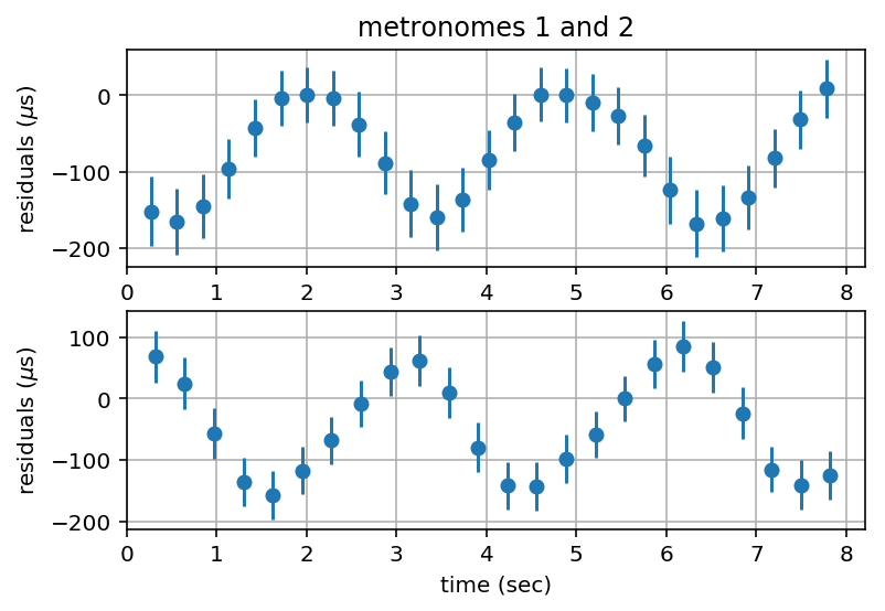
Plot Residuals
tlim = 1.05*max(residuals1[-1,0],residuals2[-1,0])

plt.figure()
plt.subplot(2,1,1)
plt.errorbar(residuals1[:,0], 1.e6*residuals1[:,1], 1.e6*errorbars1[:,1], fmt='o')
plt.xlim(0, tlim)
plt.ylabel('residuals ($\mu$s)')
plt.title('metronomes 1 and 2')
plt.grid('on')

plt.subplot(2,1,2)
plt.errorbar(residuals2[:,0], 1.e6*residuals2[:,1], 1.e6*errorbars2[:,1], fmt='o')
plt.xlim(0, tlim)
plt.xlabel('time (sec)')
plt.ylabel('residuals ($\mu$s)')
plt.grid('on')
plt.draw()
Fit Sinusoid with Constant Offset to Residuals and Plot
# default parameter choices
p1 = 2e-4
p2 = 0.4
p3 = 0
p4 = 0

#p1, p2, p3, p4  = input('input guess for amplitude, freq (Hz), phase (rad), offset (sec) for metronome 1: ')
pars1 = np.zeros(4)
pars1[0] = p1
pars1[1] = p2
pars1[2] = p3
pars1[3] = p4

pfit1, pcov1, infodict, message, ier = opt.leastsq(tpta.errsinusoid, pars1, args=(residuals1[:,0], residuals1[:,1], errorbars1[:,1]), full_output=1)

# default parameter choices
p1 = 2e-4
p2 = 0.4
p3 = 0
p4 = 0

#p1, p2, p3, p4  = input('input guess for amplitude, freq (Hz), phase (rad), offset (sec) for metronome 2: ')
pars2 = np.zeros(4)
pars2[0] = p1
pars2[1] = p2
pars2[2] = p3
pars2[3] = p4

pfit2, pcov2, infodict, message, ier = opt.leastsq(tpta.errsinusoid, pars2, args=(residuals2[:,0], residuals2[:,1], errorbars2[:,1]), full_output=1)

# best fit sinusoids
tfit = np.linspace(0, max(residuals1[-1,0], residuals2[-1,0]), 1024)
yfit1 = pfit1[0]*np.sin(2*np.pi*pfit1[1]*tfit + pfit1[2])
yfit2 = pfit2[0]*np.sin(2*np.pi*pfit2[1]*tfit + pfit2[2])

# constant offsets
N1 = len(residuals1[:,0])
N2 = len(residuals2[:,0])
offset1 = pfit1[3]*np.ones(N1)
offset2 = pfit2[3]*np.ones(N2)

# plot residuals with constants removed and with best fit sinusoids
plt.figure()
plt.subplot(2,1,1)
plt.errorbar(residuals1[:,0], 1.e6*(residuals1[:,1]-offset1), 1.e6*errorbars1[:,1], fmt='o')
plt.plot(tfit, 1.e6*yfit1, 'r-')
plt.xlim(0, tlim)
plt.ylabel('residuals ($\mu$s)')
plt.title('metronomes 1 and 2')
plt.grid('on')

plt.subplot(2,1,2)
plt.errorbar(residuals2[:,0], 1.e6*(residuals2[:,1]-offset2), 1.e6*errorbars2[:,1], fmt='o')
plt.plot(tfit, 1.e6*yfit2, 'r-')
plt.xlim(0, tlim)
plt.xlabel('time (sec)')
plt.ylabel('residuals ($\mu$s)')
plt.grid('on')
plt.draw()

# print to file
plt.savefig(tsfile + "_residuals.pdf", bbox_inches='tight')
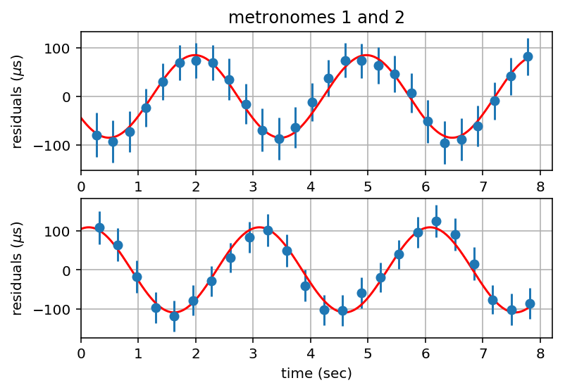
Calculate Correlation Coefficient
rhox, rhoy, rhoxy = tpta.calcorrcoeff(yfit1, yfit2)
print('correlation coeff = ', rhoxy)
correlation coeff = -0.724534807671